Benchmarking Loop Scheduling Algorithms in OpenMP
In this blog post, we’ll experiment with two loops in C which we call L1 and L2. We run L1 and L2, measure their execution time and analyse our captured performance results. Using OpenMP and its parallel for-loop directive, we will parallelise L1 and L2.
We run the code on Cirrus, one of the EPSRC Tier-2 National HPC Facilities in the UK, with 280 standard compute nodes and 38 GPU compute nodes. Here, we use the CPU nodes with two Intel Xeon Broadwell (2.1 GHz, 18-core) and 256 GiB of memory per CPU node. If you haven’t heard about it yet, as an academic in the UK you can apply for access to Cirrus but you should be able to reproduce our results on any multi-threaded machine with OpenMP.
The code can also be found on GitHub.
In OpenMP, we use the following schedule options: static, auto, static with chunksize n, dynamic with chunksize n and guided with chunksize n. First, we run the code on four threads with chunksizes n = 1, 2, 4, 8, 16, 32, 64 and determine the best schedule option for each loop. The best schedule option is defined as schedule option with the shortest execution time. Second, we run each loop with its best schedule option on different numbers of threads m = 1, 2, 4, 6, 8, 12, 16.
Let’s get started. First, we have a look at the source code and its most important elements. Then we dive into our experimentations and capture results. We present results for runtime performance and speedup of the various schedule options. Once we’ve gathered performance results, we analyse the schedule options with L1’s and L2’s workload distribution in iterations. Finally, we summarise our observations with conclusions.
Code
For both loops the given source code runs 729 iterations as indirectly defined at the file’s top (line 3, Listing 1) and later used in the loop declaration (line 6, Listing 2 resp. line 9, Listing 3).
  ...

  #define N 729
  #define reps 1000

  ...

  for (r=0; r<reps; r++){
    loop1();
  }

  ...

  for (r=0; r<reps; r++){
    loop2();
  }

  ...
L1 and L2 are executed 1000 times or repetitions, defined at the file’s top (line 3 and 4 in Listing 1). The execution time for 1000 executions is captured.
We add the OpenMP directive parallel for to the code (line 4, Listing 2 and line 7, listing 3). The parallel keyword spawns a group of threads in a parallel region and for divides the loop iterations between these threads. Moreover, we declare default(none) and explicitly declare all the variables used inside the following outermost for-loop.
void loop1(void) {
  int i,j;

  #pragma omp parallel for default(none) shared(a, b) private(i, j) schedule(guided, 8)

  for (i=0; i<N; i++){
    for (j=N-1; j>i; j--){
      a[i][j] += cos(b[i][j]);
    }
  }

}
For L1 we define the nested loops’ counters i and j as private to ensure each thread initializes its own copy. In L1 the code reads from array b (line 8, Listing 2) and writes to array a. Both arrays are initialized outside the parallel for. As all of the spawned threads should read from and write to the same arrays a and b, we declare a and b as shared. The code does not involve race conditions with reading from and writing to these arrays as each iteration targets a distinct array index. The best schedule option for L1 is guided with chunksize n=8.
void loop2(void) {
  int i,j,k;
  double rN2;

  rN2 = 1.0 / (double) (N*N);

  #pragma omp parallel for default(none) shared(b, jmax, rN2, c) private(i, j, k) schedule(dynamic, 16)

  for (i=0; i<N; i++){
    for (j=0; j < jmax[i]; j++){
      for (k=0; k<j; k++){
        c[i] += (k+1) * log (b[i][j]) * rN2;
      }
    }
  }

}
A similar approach is taken for L2. We define the nested loops’ counters i, j and k as private, again to ensure reliability and prevent one thread’s counting from having impact on another thread’s counting. For the used variables in L2’s nested loops we want the threads to read and write to the same arrays or from variables with the same value, thus we declare b, jmax, rN2 and c as shared. Again, the loops and their iterations read and write to distinct array indices (line 12, listing 3). t
Therefore, we do not have to worry about race conditions. The best schedule option for L2 is dynamic with chunksize n=16.
Results
This section presents our observations from parallelisation with the different schedule options on the execution times of L1 and L2. These observations are discussed in the following section 4 Analysis.
| Schedule option | L1 execution time [sec] | L2 execution time [sec] |
|---|---|---|
| Static | 0.719 | 6.216 |
| Auto | 0.433 | 5.457 |
Chunksizes on L1
Figure 1 visualises the execution time for the schedule options static, n, dynamic, n and guided, n on L1. With the exception of n=2, static, n always takes longer execution times than dynamic or guided. For n=2 we observe a by 0.001 seconds longer execution time with the schedule option dynamic, n than with static, n. For guided and dynamic, n the execution time rises by ca. 0.015 seconds from n=1 to n=2 while for static, n the execution time decreases by 0.01 seconds. In general, execution time on L1 for chunksizes n=1, 2, 4, 8, 16, 32, 64 is the shortest for guided, n, followed by dynamic, n and with static, n having the longest execution time. Comparing dynamic and guided, we can see that from n=1 to n=16 the difference in execution time decreases, whereas from n=16 to n=64 the difference between the three schedule options increases.
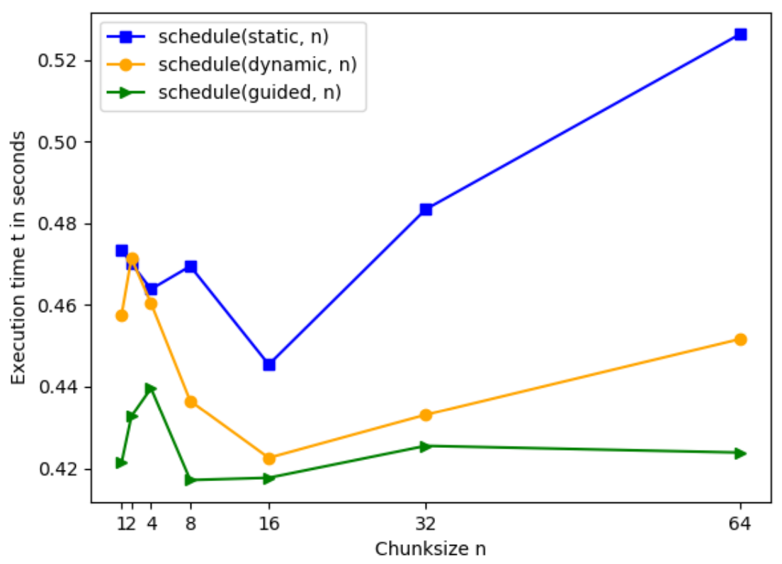
With the increase in chunksize from n=1 to n=4 the execution time of guided rises sharply from 0.421 seconds to its maximum of 0.439 seconds, then considerably falls to its minimum of 0.417 seconds at n=8. From n=8 to n=32 execution time slightly rises to 0.425 seconds and afterwards declines to 0.423 at n=64.
Dynamic’s execution time increases from 0.458 seconds at n=1 to 0.471 seconds at n=2 and reaches its maximum in our observations. Thereafter, execution time drops to 0.436 at n=16. From n=16 to n=64 it grows again to 0.452 seconds.
The execution time of static is 0.473 seconds at n=1, then it fluctuates and goes down to 0.445 seconds at n=16. From this minimum it rises to 0.526 seconds at n=64.
Chunksizes on L2
The execution time for static, n, dynamic, n and guided, n on L2 is illustrated in Figure 2. For chunksizes n=1,2,4,8,16,32,64 the schedule option that takes the shortest execution time is dynamic, n, followed by static, n and guided, n. The shape of static, n’s and dynamic, n’s graphs look similar. Both execution times decrease from n=1 to n=8, then sharply rise with similar rate from n=8 for static, n and from n=16 to n=32 for dynamic, n.
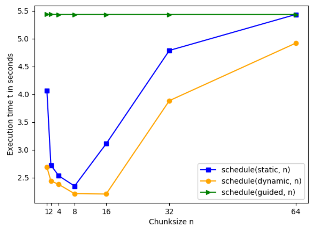
From 2.687 seconds at n=1 the execution time of dynamic, n drops to 2.211 seconds at n=8. Execution time slightly decreases from n=8 to n=16 to 2.205 seconds. From n=16 to n=64 it increases strongly by 2.616 seconds to 4.921 seconds.
At n=1 execution time for static, n takes 4.064 seconds and falls by 1.241 seconds to n=2, decreases further to 2.348 seconds at n=8 reaching its minimum. From n=8 to n=64 execution time rises to 5.436 seconds.
Guided takes the longest execution time on L2 for chunksizes n and only fluctuates between 5.436 seconds and 5.437 seconds.
Threads
From our observations we determine the best schedule option with chunksize n for L1 and for L2. For L1 the schedule option with the shortest execution time on four threads is guided, n=8, for L2 it is dynamic, n=16. We run these schedule options for the respective loops on m=1,2,4,6,8,12,16 threads. Figure 3 shows the execution time against the number of threads for L1 and L2.
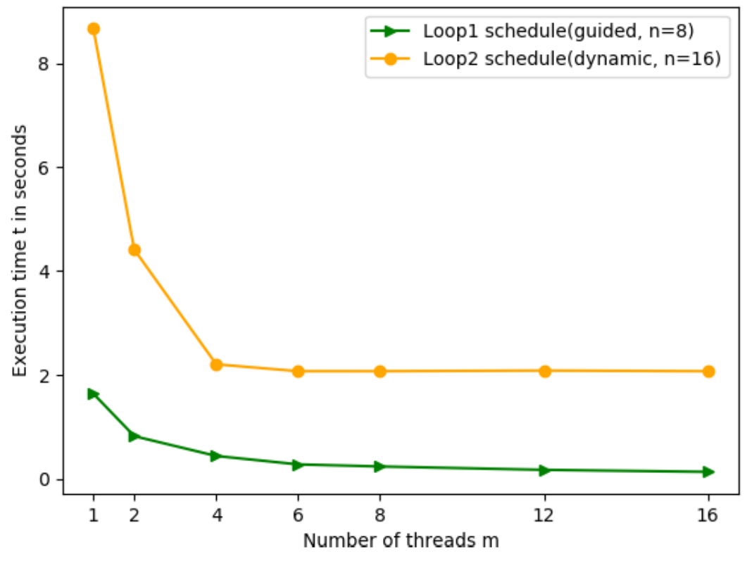
For L1 and L2 the execution times decrease in the number of threads m. For L1 the execution time decreases sharply from 1.632 seconds at m=1 to 0.828 seconds at m=2. From m=2 to the increased numbers of threads m the execution time decreases further but less steeply to 0.188 seconds at m=16. With m=1 the execution time for L2 amounts to 8.741 seconds. Increasing the number of threads to m=2 we observe a substantial decrease to 4.438 seconds at m=2 and execution time keeps falling sharply to 2.238 seconds at m=4. From m=4 to m=16 the execution time decreases slightly by less than 0.011 seconds.
Speedup
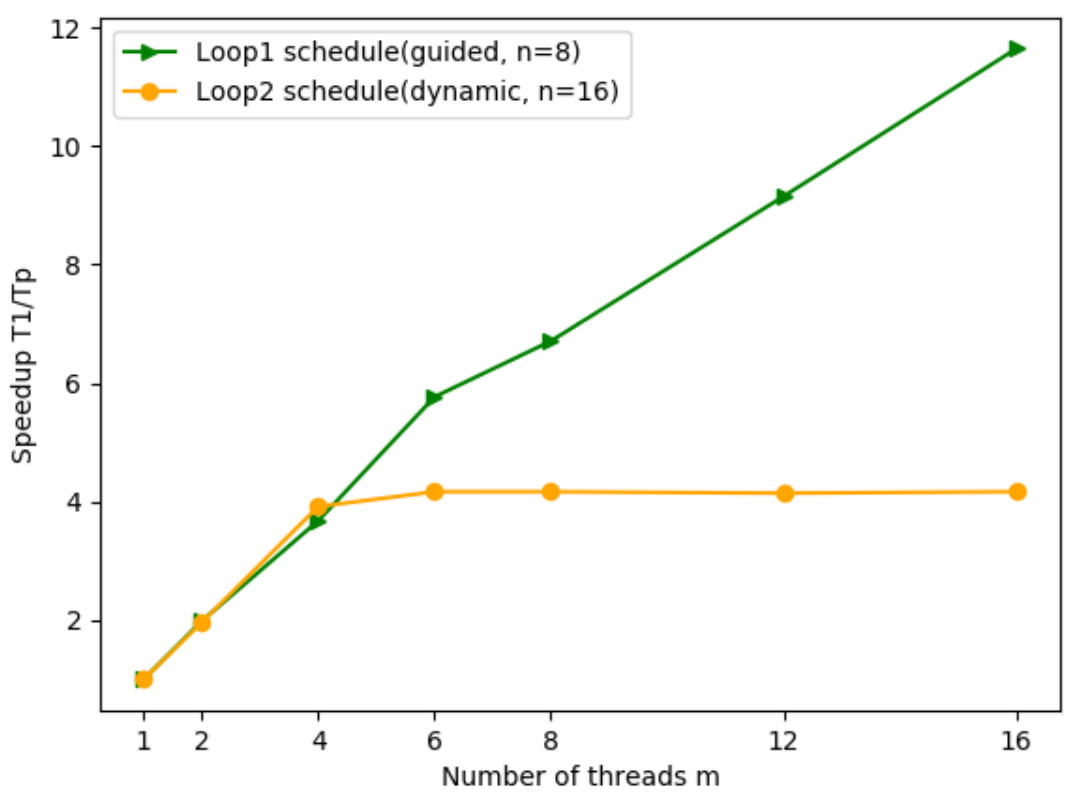
The speedup is defined as s = T1/Tp with execution time in serial T1 and execution time on p processes Tp. Figure 4 shows the speedup against the number of threads m. L1 shows an approximately linear increase in m from s=0.9 at m=1 to s=5.9 at m=6. From s=5.9 at m=6 its speedup increases further with decreased gradient to s=11.8 at m=16. Similarly, L2’s speedup increases from s=0.9 at m=1 to s=4.0 at m=4. From s=4.0 at m=4 to m=16 the speedup does not increase significantly and keeps its level of s=4.0.
Analysis
Suitability and potential performance gain of the schedule options differ. To discuss what type of schedule option leads to increase or decrease in execution time on L1 and L2, we first need to understand the schedule options’ general behaviour and secondly have to analyse L1’s and L2’s distribution of workload over iterations.
Schedule options
For balanced loops with stable workload throughout their iterations static (without chunksize) is preferred as this option includes the least overhead in allocating equally sized chunks of iterations to an a priori known number of threads. With defined chunksize, static, n allocates chunks of chunksize n to threads in cyclic order.
The more often a loop is executed the more advantageous is the auto schedule option. With an increasing number of executions, runtime can develop well balanced schedules. The implementation how runtime achieves optimisation depends on factors like compiler and hardware.
With dynamic schedule option, iterations are allocated to threads in chunks of chunksize n on a first-come-first-served basis. The thread that finishes first is assigned with the next chunk. This schedule option is useful for loops of diverging workloads in iterations.
Schedule option guided suits loops of gradually decreasing workloads in iterations. It allocates iterations chunks of varying size to threads, also on a first-come-first-served basis. The initial chunksize is large and it declines exponentially to the minimal size of n.
Workload distribution in L1
L1 consists of an outermost for-loop with counter i (line 6, Listing 2) and one nested for-loop with counter j (line 7, Listing 2). i counts up from 0 to 728<N. j counts down from N-1=728 to i+1 (or while j>i). Thus, i depends on N and j depends on i. The statement on line 8 in Listing 2 is only executed while j is larger than i. This illustrates that with every increase in i there are less iterations of the nested loop. In summary, L1’s workload (execution of line 8 in Listing 2) decreases linearly in the outer loop’s iterations (or with an increase in i).
Workload distribution in L2
L2 includes an outermost for-loop with counter i (line 9, Listing 3), a nested for-loop with counter j (line 10, Listing 3) and one innermost for-loop with counter k (line 11, Listing 4). i depends on N, j depends on jmax[i], jmax[i] depends on i and i\%( 3*(i/30) + 1), and k depends on j. Again, i counts up from 0 to 728<N. j counts up from 0 while j<jmax[i]. The array jmax is initialised in init2() and its item values are either N=729 or 1. If the right side of statement expr = i\%( 3*(i/30) + 1) evaluates to 0 then jmax[i] is assigned with the value 0 otherwise jmax[i] is assigned with value 1. The pattern introduced by expr leads to an iteration for all of the first 30 values of i. Counting up from i=29 the nested loop leads to a gradually decreasing number of iterations with in-between peaks, dependent on the expr-pattern. The innermost loop counts up from 0 while k<j, thus further increasing the dependence on j respectively jmax[i]. Summarising, L2’s workload decreases gradually in i with exceptions following a pattern dependent on expr.
Comparison
Option auto does a decent job in developing adjusted schedules and is expected to increase its absolute advantage with an increasing number of repetitions. For dynamic, it is similar to guided: To a certain point this schedule option holds advantage on its flexible allocation of chunks to idle threads. Compared to guided, dynamic does not reflect L1’s special characteristic of decreasing workload in iterations. Instead, dynamic always assigns the same chunksize, resulting in higher execution times with heavily increasing chunksizes.
Generally, Static is not suitable for imbalanced loops like L1. This schedule option assigns a (default) chunksize to the available number of threads. With imbalanced loops static leads to non-utilised idle threads resulting from earlier finished processes because of different thread workloads. Depending on chunksize static’s execution time decreases, leading to on observed minimum.
The option guided fluctuates around a small corridor of execution time. It neither substantially decreases its execution time over chunksize n nor does it increase execution time. This stems from its gradually decreasing chunksize while L2 comprises emerging workload peaks spread all over its iteration space. For the tested chunksizes, guided is substantially worse at handling the workload pattern of L2 than the other chunksize schedules. Option auto fails at evolving a balanced schedule on L2 as its workload is never equally spread over its iterations space. Static with default chunksize leads to idle threads an inefficient workload allocation. Static with small chunksizes is able to take advantage of a low average of iteration workload as the distance between high-workload iterations increases in i. With increasing chunksize this advantage diminishes.
Conclusion
The decreasing workload in i for L1 fits the schedule option guided, n. For small numbers of n, there exists increasing overhead in allocating small chunks to threads. With an increase in chunksize (for guided chunksizes start off large and decrease to minimum chunksize n), this overhead reduces to an observed minimum of execution time. In general, guided handles L1’s workload best as L1’s declining workload suits guided’s initially high and gradually decreasing chunksizes. L1’s linearly decreasing workload is reflected in its approximately linear speedup for guided, n=8.
L2 comprises a gradually decreasing workload in iterations with emerging peaks in between. It is an imbalanced loop and compared to L1 it consists of an unsteady pattern (or workload gradient) in i. With its flexibility in assigning chunks to idle threads, schedule option dynamic achieves the shortest execution time but is not able to foster further speedup with more than 4 threads, illustrated in Figure 4. On L2, the option is more efficient for smaller chunksizes as the distance between high-workload iterations increases in i. The bigger the chunksize, the higher the increase in execution time.
What’s next?
Now that we’ve looked at the various scheduling algorithms in OpenMP, let’s think about an alternative implementation: Facing unbalanced workload distribution, could we implement a work-stealing mechanism in the sense that once a thread finishes its local workload, it starts picking workload chunks from the thread with the currently highest remaining workload? We call this Affinity scheduling and we will have a closer look at this approach in the next blog post on Developing an Affinity Scheduling Algorithm.