Developing an Affinity Scheduling Algorithm
This blog posts focuses on an affinity scheduling implementation in C and OpenMP.
We develop the code and benchmark our affinity scheduling approach with the two
loops L1 and L2, which we introduced in an earlier blogpost on
Benchmarking loop scheduling algorithms in OpenMP. Our experimental setup is the same as in the earlier blogpost:
We run our affinity scheduling implementation on Cirrus using
m = 1, 2, 4, 6, 8, 12, 16 threads. Remember OpenMP’s built-in scheduling
algorithms wich we compared in the mentioned blogpost? Here, we compare
execution time and speedup of our affinity scheduling approach to OpenMP’s
built-in schedules.
Follow along the tutorial or run the code by yourself - find it on GitHub.
How does the Affinity Scheduling Algorithm work?
Initially, the affinity scheduling algorithm distributes loop iterations across processes. Threads running idle after having processed their assigned chunks start picking a chunk from the remaining, most loaded thread’s iterations until all iterations are processed.
Let’s develop the code: First, we describe our algorithm with its data structures and the required synchronisation to avoid race conditions which could falsify our results. Secondly, we explain our experimental results and compare them to OpenMP’s built-in schedule options and their performance before we dive deeper into our analysis. Finally, we summarise our outcomes and present conclusions.
Affinity scheduling algorithm
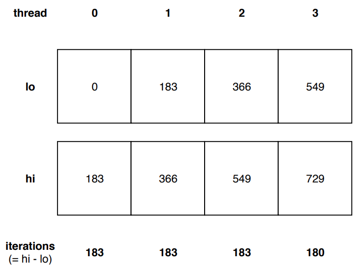
Our affinity scheduling algorithm relies on two shared arrays that we
initialise before spanning a parallel region. lo and hi carry the
initial lower respective higher boundaries indexed by thread ID.
Spanning the parallel region, each thread computes its part out of the
total number of iterations N. Table 1 shows the initial allocation of
iterations to threads for N=729 iterations.
Initial allocation of N=729 iterations:
| Threads P | 1/P | 1/P * N | IPT |
|---|---|---|---|
| 2 | 0.500 | 364.5 | 365 |
| 4 | 0.250 | 182.3 | 183 |
| 6 | 0.167 | 121.5 | 122 |
| 8 | 0.125 | 91.1 | 92 |
| 12 | 0.833 | 60.8 | 61 |
| 16 | 0.063 | 45.6 | 46 |
A thread is assigned with a
fraction 1/P of N iterations. We round this fraction up to the next
integer number of iterations. Ideally, each thread is assigned an equal
number of iterations. As we round the fraction up to IPT we have to
assure that no thread’s hi boundary is larger than N, occasionally
resulting in a lower difference between the last assigned thread’s hi
and lo boundaries compared to its neighbours. Figure 2. shows the
boundaries’ data structure for four threads and 729 iterations.
Synchronisation
After locally computing boundaries hi and lo we synchronise threads
before spanning a critical region. Our boundary arrays are shared over
threads and each thread sets its own initial boundaries. Before checking
for local or global available chunks the program has to wait for all
threads to have their boundaries set. Our boundary arrays serve as
single point of truth for the calculation of chunksizes in either case:
Processing a thread’s own chunks or the (currently) maximum loaded
thread’s chunks. We use a #pragma omp barrier statement to synchronise
threads. With this barrier we have a global set of current boundaries
from which we derive available chunks and a thread’s target chunksize.
Critical region
Introducing a critical region we anticipate race conditions within our
algorithm. Each thread reads from both boundaries, calculates a
chunksize from these and writes a new, increased value to
lo[thread_id]: lower boundary + new chunksize to process = new lower boundary.
Inside the parallel region we confine our algorithm’s look-up and chunksize calculation parts. Synchronised threads enter a while loop whose condition holds true as long as there are chunks globally available.
Figure 2 presents the algorithm’s critical section in Business Process
Model Notation 2.0 (BPMN). Each thread checks if there still exists
remaining chunks for its ID. If there are chunks available the thread
will use its own ID to target these chunks. Otherwise, the thread
iterates over the global set of boundaries and computes the maximum
loaded thread’s ID to derive a chunksize and an update to
lo[target_id].
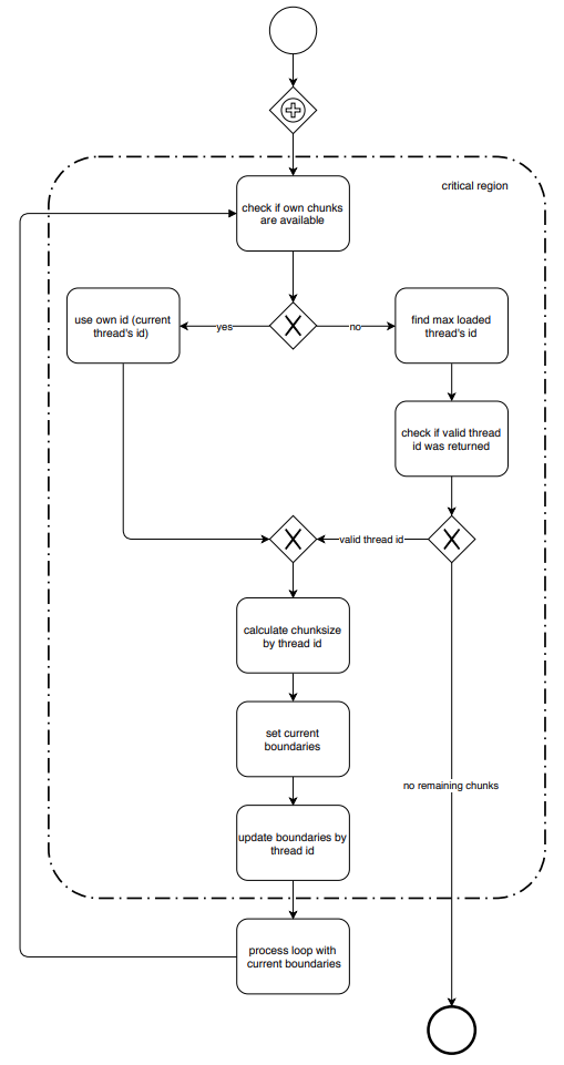
If the global set of iterations is finished the search for the maximum
loaded thread will lead to an invalid thread ID and the while loop’s
condition will no longer hold true. The program leaves the critical
region and returns to main.
Based on either its own thread ID or on a valid thread ID returned from
the maximum workload search, the thread reads the boundaries, derives a
chunksize, sets the current boundaries to process for
loop1chunk(current_lo, current_hi) or
loop2chunk(current_lo, current_hi) and updates the global boundaries.
In our implementation we continuously write to the lower boundary array
lo[] while the upper boundary hi[] stays constant and untouched
after initialisation. The algorithm computes chunksizes of fraction
ceil(1/P * (hi[target_id] - lo[target_id]) until no remaining
iterations are available.
After updating the boundary the program leaves the critical region to perform the previously defined iterations of either L1 or L2. While the current thread executes the calculations inside the for loop, other threads are allowed to enter the critical section - one thread at a time.
Finishing the for loop’s iterations the thread reaches the while loop’s end and the while loop’s condition is checked, again. Having processed a for loop with current boundaries, the thread faces a while loop condition that still holds true. The process starts again and is executed until the search for the maximum loaded thread returns an invalid thread ID.
Results
We use our performance data from Benchmarking loop scheduling algorithms in OpenMP and compare the results of OpenMP’s built-in schedule options to the performance of our implementation of the
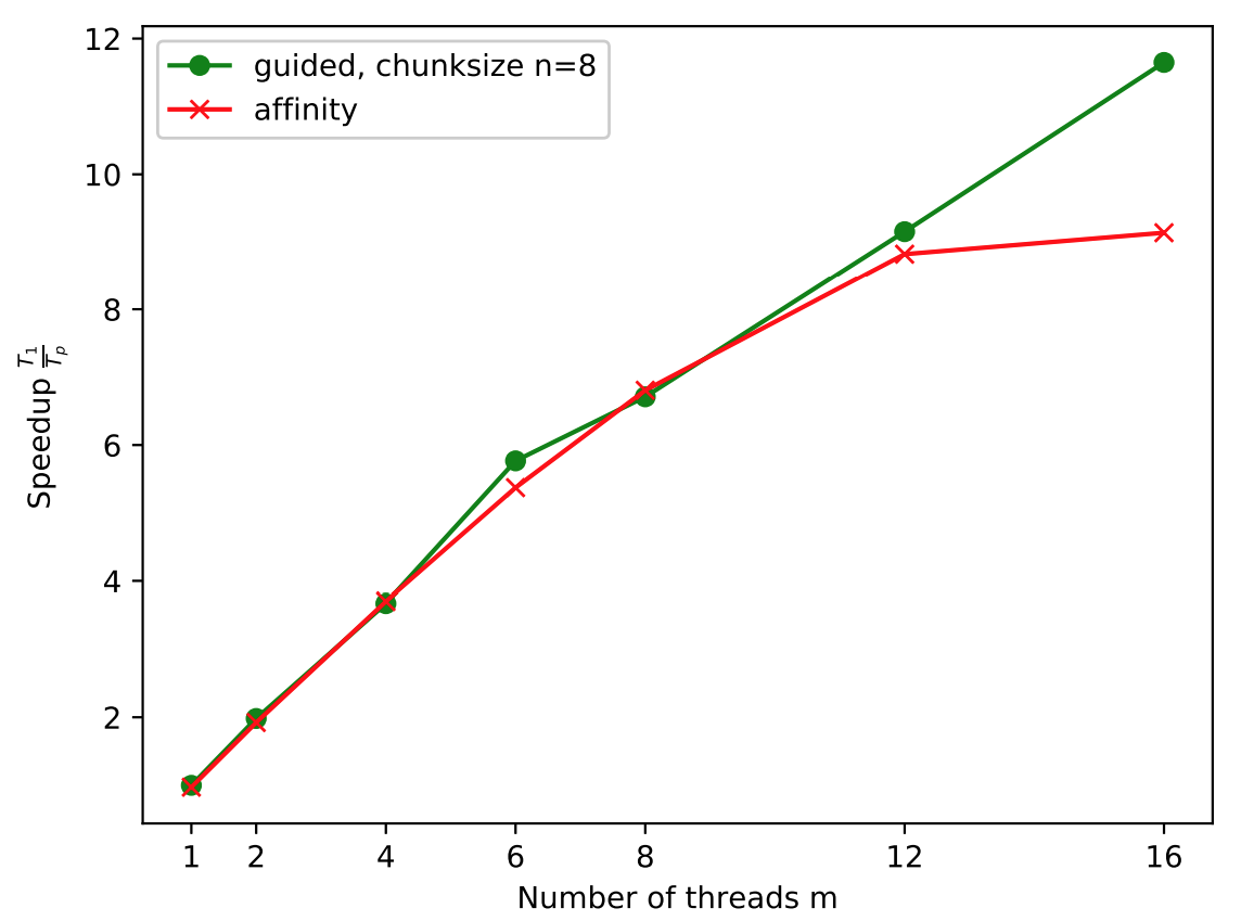
affinity scheduling algorithm. The best previously identified schedule
options are guided with chunksize n=8 for L1 and dynamic with
chunksize n=16 for L2. We run the code on m=1, 2, 4, 6, 8, 12, 16
threads.
The affinity scheduling implementation’s execution time in Figure 1 halves from serial to two threads.
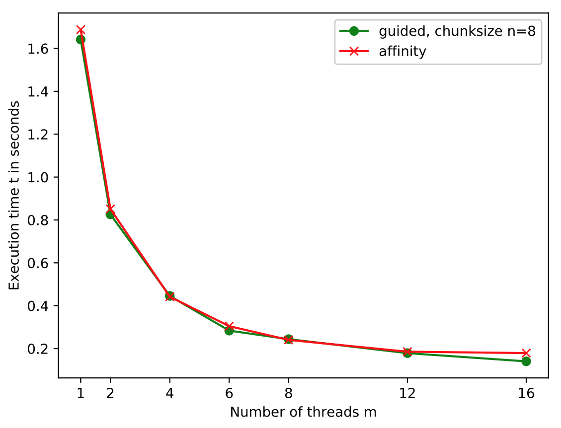
Increasing the number of threads, the
execution time decreases further but shows falling slopes. From m=2 to
m=4 the execution time halves again. From m=4 to m=12 the overhead
plunges by about 50%. Comparing affinity to guided, 8 we observe
similar execution time for increasing number of threads. While guided
decreases to about 0.152 seconds at m=16, affinity’s execution time
falls slightly less.
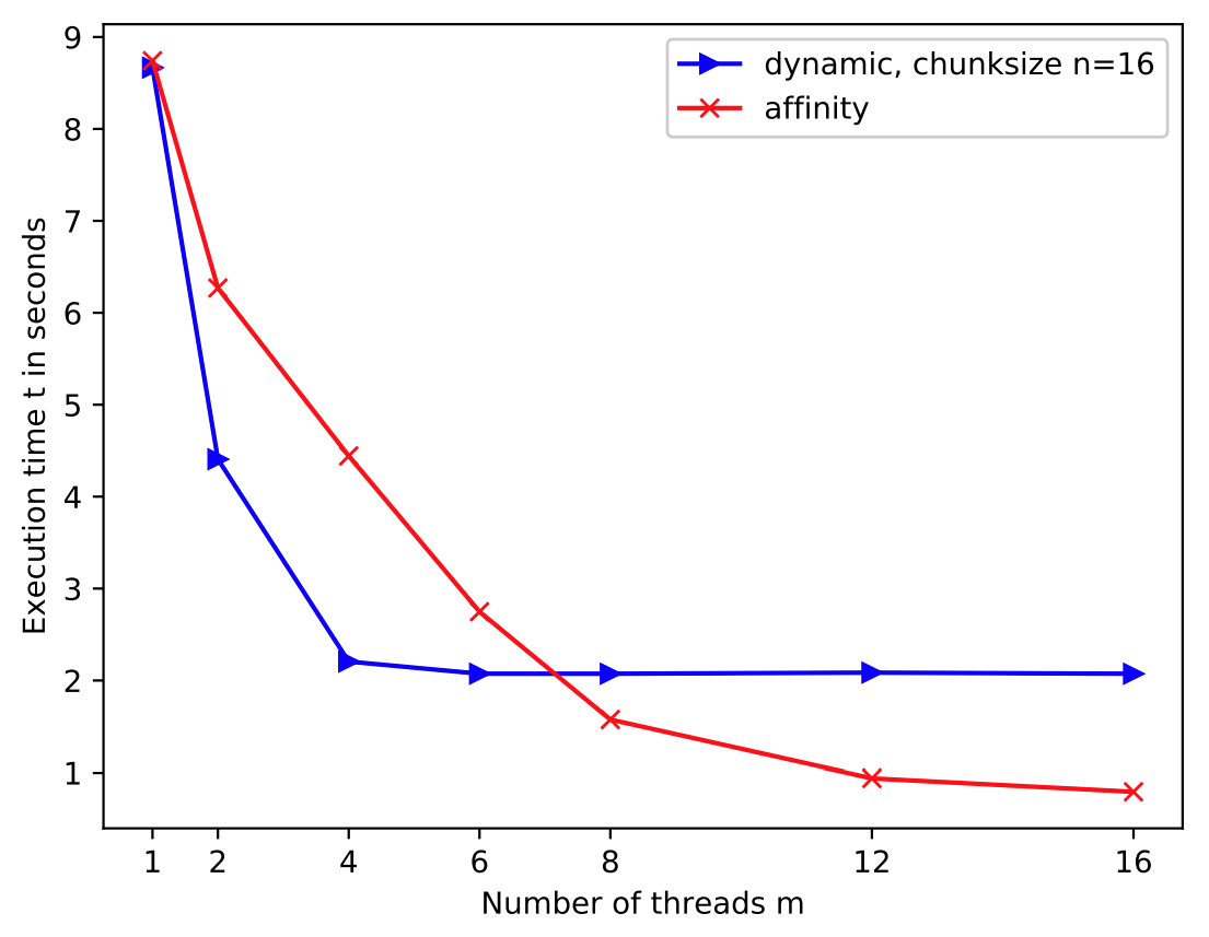
The execution time on one thread takes about 8.8 seconds for affinity.
Figure 3 shows that our implementation halves its execution time from m=1 to
m=4 threads. From m=4 to m=8 our affinity algorithm’s execution
time falls from 4.5 seconds to about 1.6 seconds. Increasing m
further, leads to falling execution time with less steep slope. Compared
to dynamic, 16 the algorithm includes higher overhead from m=1 to
m=6. dynamic’s execution time stays about constant from m=4 to
m=16 while affinity decreases its overhead to less than a second on
16 threads.
Analysis
As our observations in reducing execution time suggested, affinity
comprises a nearly ideal speedup for well-balanced loop L1, shown in
Figure 2.
The overhead for smaller number of threads is marginal. Experimenting without atomic, locks or critical regions we observed intervals of correct calculations and results. Increasing numbers of threads eventually lead to higher overhead concerning waiting time in front of our implementation’s critical region.
Schedule option dynamic starts off with higher chunksizes than our
affinity implementation, resulting in a higher speedup from m=1 to
m=6. Thereafter, L2’s imbalanced workload distribution leads to idle
threads if used with schedule option dynamic. Affinity’s threads
face a critical region but their decreasing chunksizes and the
algorithm’s general intention comprises idle threads to pick up foreign
threads’ remaining workload.
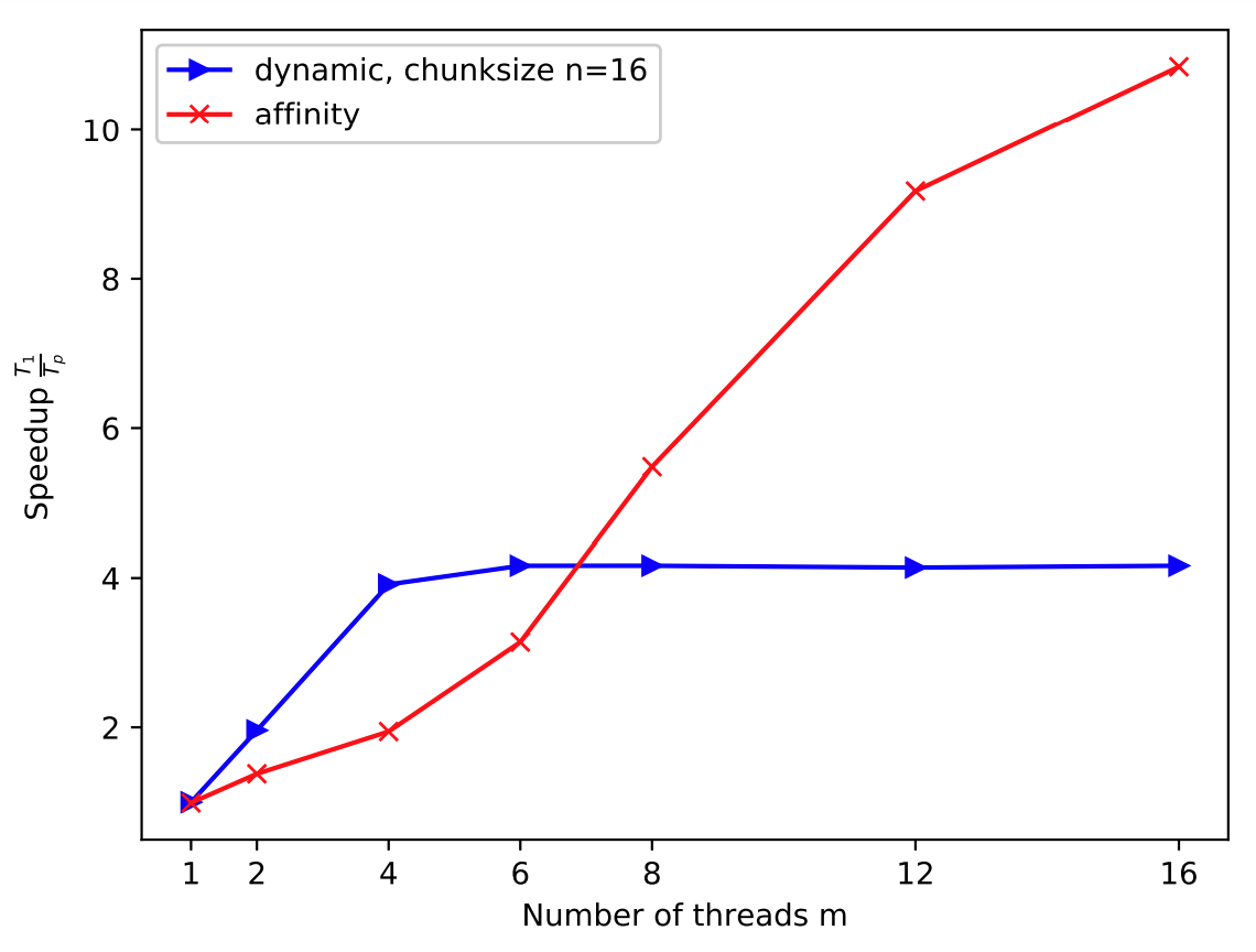
An increasing number of threads leads to higher speedup for affinity
on L2. L2 is an imbalanced loop with highly varying chunksizes in its
iteration set. While dynamic's threads might run idle for longer
periods, compared to affinity, our implementation’s threads keep
constantly searching for foreign chunks if they finished processing
their own locally assigned sets of iterations. The unsteady workload
distribution for L2 could foster affinity’s performance as threads
that were initially assigned low-loaded chunks act as periodic workload
facilitators. Figure 4 shows an constantly rising speedup for
affinity.
As long as the imbalanced workload distribution of L2 does not cause too
many threads running idle, respectively finishing their local iterations
chunks, speedup for affinity irresistibly rises. The more imbalanced
the loop, the higher the advantage of affinity compared to dynamic
or other built-in OpenMP schedule options. We expect increasing
overheads for affinity with massive numbers of threads. This effect is
promoted by balanced loop with equally distributed workload over
iterations. The more threads start searching for foreign chunks at the
same time or within very small time series, the higher the overhead for
our affinity implementation.
Conclusions
From our algorithm implementation and the conducted experiments we derived conclusions concerning race conditions, data structures, synchronisation and performance.
Race conditions
Writes to shared variables are nasty and OpenMP provides distinct tools
to manage them adequately. For the algorithm and data structure, we have
to make sure that read and writes to the global boundary arrays lo[]
and lo[] work correctly. Having two threads writing to the same
boundary at the same time, i.e. lo[1] could lead to a successful write
of thread 1 and an aborted or unsuccessful write of thread 2, or vice
versa. Reading on thread 2 from lo[1] while writing to this item could
similarly lead to obscure outcome. OpenMP offers critical and atomic
directives to resolve this conflict. The latter is very handy for single
write statements. Generally, atomic involves less overhead and better
performance than critical. Trading-off implementation ideas we ran
quick tests whose outcome underpin this statement.
Nevertheless, our implementation of the affinity scheduling consists of
a more complex background. The race condition that we observed was not
resolved by single atomic statements to the write and reads of lo[]
and hi[]. The race condition was a combination of concurrent access
and time difference between two of the algorithm’s main functionalities.
Searching through the boundary arrays for the maximum loaded thread, a
thread must have access to a reliable chunk glossary.
Two threads 0 and 2 accessing the boundary arrays at the same time, or
slightly after each other, find the same maximum work loaded thread.
Thus, both threads calculate the same chunksize, write the same value
update to lo[] and perform redundant iterations falsifying our result.
Table race_condition_table shows a situation with four threads.
Threads, their local chunks and targeted threads (max. load thread resp. own ID):
| Thread | hi - lo | Target |
|---|---|---|
| 0 | 0 | 1 |
| 1 | 5 | 1 |
| 2 | 0 | 1 |
| 3 | 4 | 3 |
Thread 0 and 2 finished their local iterations and target the most loaded thread: Thread 1. Thread 1 and 3 work on their local sets of iterations as the difference of their boundaries specifies remaining chunks. Figure 7 illustrates the situation on a timeline.
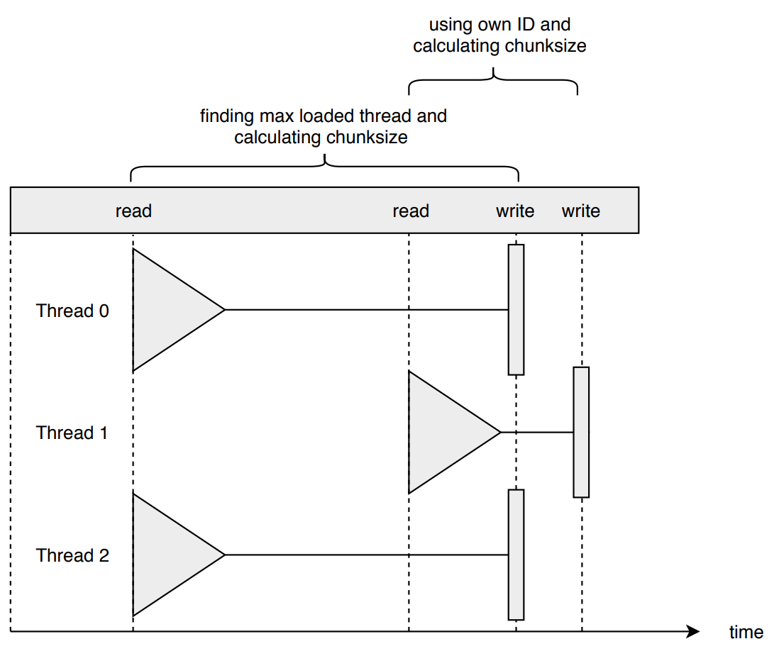
First, searching for the most loaded thread requires reading lo[] and hi[].
Threads 0, 1 and 2 target the same chunks of thread 1. Thread 0 and 2
read its boundaries at the same time. Having found their target both
threads seek to write to lo[1] to decrease the amount of remaining
iterations for thread 1. Thread 1 reads its boundaries at a later point
in time than thread 0 and 2 but before its competitors finished their
write to thread 1’s lower boundary. All of these three threads obtain
the same chunksize with identical iterations resulting in redundant
executions of iterations and a wrong calculation output.
Critical regions and performance
To prevent wrong results and redundancy, the depicted pair of actions in
Figure 7 need to be performed by one thread at a time and in successive
order without interruption by other threads. OpenMP’s critical
directive is a suitable solution. It restricts the code to one thread at
a time and eliminates the race condition. Putting both action pairs
finding max loaded thread and calculating chunksize and
using own ID and calculating chunksize in this critical region as in
Figure 2 led to correct, reproducible and stable results.
From a theoretical point of view, the critical region is a necessary
performance bottleneck as only one thread at a time is allowed to
perform search and chunksize computation; there is no performance
tradeoff against correct code. Our analysis shows that for L1 the
affinity scheduling implementation performs similarly good as the best
built-in option guided, 8. For L2, the algorithm performs better in
increasing number of threads. We estimated that with increasing number
of threads the overhead in waiting for entrance to the critical region
rises. With the data obtained during experimentation we cannot be
sufficiently sure about the increasing overhead. Figure
2 indicates
that for a well-balanced loop like L1 the speedup rises less steeply for
an increase form m=12 to m=16 threads. Further experimentation could
capture the overhead for waiting in front of the critical region and the
time spent inside it. Capturing the time one could make use of OpenMP’s
reduction directives.
Data structures and synchronisation
At the beginning of our algorithm we locally compute a thread’s
allocation of the overall number of iterations and set up its
boundaries. Developing our code and experimenting with low numbers of
iterations N, we occasionally observed diverging results.
Synchronising threads after they declared their correct boundaries with
the shared variables hi[] and lo[], we were able to resolve this
issue. With an increasing number of threads and computation across
multiple nodes it is likely that the number of wrong calculations rises
if there is no synchronisation. Omitting synchronisation after initial
boundary setup could cause wrong results during the search for the
maximum work load. If threads have not set their boundaries by then, the
underlying search functionality derives a target_id based on an
incomplete set of boundaries, thus on a non-reliable work load
reference.