Parallel Image Reconstruction
In this blog post, we will cover the application of an edge detection algorithm with two-dimensional domain decomposition implemented in C and MPI. We set up an MPI program to distribute the input image across processes in a Cartesian topology, to parallelise calculations for edge detection on these processes and communicate halos between processes across the network. Finishing calculations for edge detection processes send their results back to root that handles IO locally. Root writes a final image to filesystem.
We present non-blocking communications, boundary conditions, a stopping criterion and average pixel value calculations. Demonstrating our program’s performance we experiment with number of processes, overhead experiments and testing. Capturing time and performance we run our program on Cirrus, one of the EPSRC Tier-2 National HPC Facilities in the UK, with 280 standard compute nodes and 38 GPU compute nodes. Here, we use the CPU nodes with two Intel Xeon Broadwell (2.1 GHz, 18-core) and 256 GiB of memory per CPU node.
Btw, if you’re an academic in the UK, you can apply for access to Cirrus.
So, let’s get started. First, we introduce our program and its characteristics for image distribution, parallel edge detection and image aggregation. You can find the code on GitHub. Second, we explain our experiments and present performance results and verification tests. Third, we describe how to run our program. Finally, we summarise our findings and derive conclusions.
Code description
In our program we use MPI subroutines to parallelise the edge detection algorithm across processes. We present our framework of functionalities, data structures and how they interact.
Cartesian topology
In MPI processes are grouped in communicators. The default communicator is MPI_COMM_WORLD. Each process is assigned a rank that represents the order of processes in a communicator. By rank, we can fetch neighbouring processes for information about them and inter-process communication. Distributing the pixels of a two-dimensional image we could easily arrange the order of processes over one of the image’s dimension and split it into strips along a band. Our program’s focus is a two-dimensional decomposition as depicted in Section Image decomposition.
Setting the number of processors in our 2D communicator, we must arrange its dimensions. MPI supplies MPI_Dims_create to deal with an optimal distribution of processes in dimensions. The routine returns dims[0] and dims[1] that carry the number of processes in dimension one and two, e.g. for nine processes the routine suggests a 3x3 grid, with 3 processes in each dimension.
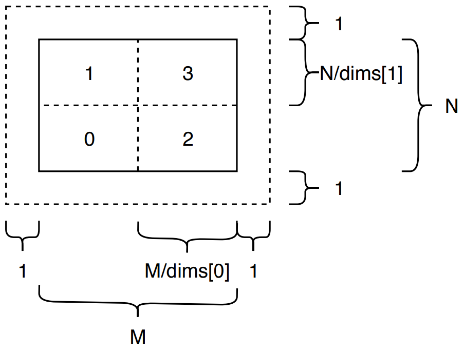
MPI conveniently provides a routine to order processes of a communicator on a two-dimensional grid. We deploy MPI’s Cartesian topology with MPI_Cart_create to span this grid of processes across our image. Figure image_size illustrates an example of four processes in a 2x2 topology.
In a one-dimensional topology, we can easily add one to the current processor’s rank to get the neighbour to the right and subtract one from current rank to receive the left neighbour’s rank. For our two-dimensional Cartesian topology we make use of MPI_Cart_shift that returns shifted ranks to the left, right, top and bottom.
Image decomposition
With the Cartesian topology in place we have a grid of processes that we assign image slices to. Reading the input edge file with pgmread from filesystem we fill a two-dimensional array masterbuf of size M times N representing the number of pixels in x- and y-dimension of a Cartesian coordinate system. Figure image_size visualises masterbuf’s split into equally sized slices. Splitting the image we calculate vertical and horizontal length of each slice. Taking previously set dimensions by MPI_Dims_create into account our slices are dynamically sized depending on the number of processes in each dimension and the image’s edge lengths.
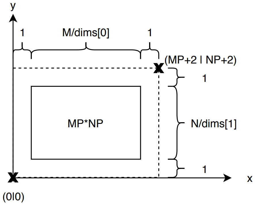
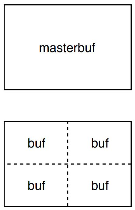
The program declares the five arrays masterbuf, buf, edge, old and new. Figure masterbuf_bufs shows the relation between masterbuf and buf for four processes on a 2x2 grid. The input image is stored in masterbuf and split into smaller slices for distribution across processes in our communicator. Manually slicing the image the program copies image slices to local buf and sends them to the destination process according to the Cartesian grid’s order of ranks. Masterbuf is of size M*N, buf has the dimensions M/dims[0] or MP times N/dims[1] or NP. The edge detection algorithm uses adjacent edge pixels from neighbouring processes. Section halo gives detailed information about the halo swap procedure. Edge, old and new implement one additional column and row on each edge to carry halo pixels. Figure edge_data_structure shows the dimensions of edge, old and new. Each of the three arrays are of size MP+2 times NP+2.
Boundary conditions
Our input edge files were created using specific boundary conditions. Reversing the operation the algorithm relies on correctly set conditions for both dimensions. Figure boundary_conditions shows the overall image’s boundary specifications. Along the x-axis or dimension one we set fixed boundaries. We declare function boundaryval that takes two input parameters to compute a returning value used to generate a saw-tooth boundary with value 255 on the right boundary’s bottom to 0 at the right boundary’s top. In between the values gradually increase. Value 255 represents white and value 0 stands for black. Gradually decreasing from 255 to 0 the value chain makes up a visual gradient with transition from white to black. The opposite image edge incorporates the equivalent saw-tooth value in reverse order.
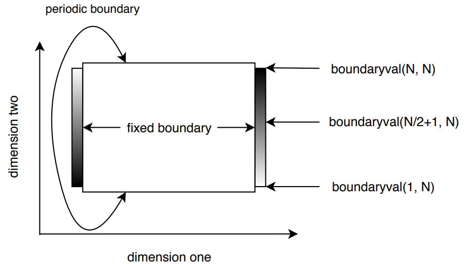
Along the y-axis or dimension two the edge images comprise a periodic boundary. Reversing the lowest pixel row at the image’s bottom in Figure boundary_conditions the algorithm relies on the highest row of pixels at the image’s top. For parallelisation, the Cartesian topology with MPI_Cart_create accepts a period parameter that we use to implement the cyclic boundary. In this implementation the top and bottom neighbours of edge processors are aligned along a cycle that enables continous halo swaping along dimension two and reflects the periodic boundary of our edge files.
Halo swaps and non-blocking communications
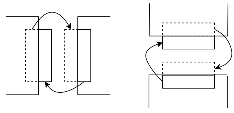
For the edge detection algorithm every pixel’s calculation relies on its four neighbours to the top, right, bottom and left. Depending on its neighbours previous pixel value, the current pixel derives its new computation value. For arbitrary pixels in the inner part of the image calculations in serial are straightforward. Parallelising and splitting masterbuf into small equally sized slices we swap halos along edges and between processes. Figure halo shows horizontal and vertical halo swaps. The outer right column of pixels of an image slice that is assigned to a specific process, dependent on the neighbouring right process’ outer left column of pixels. Image slices across processes are equally sized with MPxNP. Pre-processing the image slice we send the currents process’ outer right column to its right neighbour that receives the messages to its halo in array old[MP+2][NP+2]. For each iteration of the edge detection the current process repeats this step until halos of all its edges are swapped with its adjacent neighbours.
According to boundary conditions in Figure boundary_conditions we do not rely on halo swaps for pixels on masterbuf’s edges to the right and left as dimension one comprises fixed boundaries. Pixels on masterbuf’s edges to the top and bottom have to be swapped in cyclic order that is implemented by our Cartesian topology. Independent of the current pixel’s location on the sliced image or its location on masterbuf, our program always commits halo swaps to each four neighbours. The outer left processes in our topology do not have existing neighbours to the left and the outer right processes do not comprise neighbouring processes to their right. MPI offers MPI_PROC_NULL to resolve this conflict. Sending and receiving to or from non-existing processes MPI infers MPI_PROC_NULL that is considered a black hole. Messages send to or received from MPI_PROC_NULL are marked as successfully transmitted but do not interfere with our program’s edge detection. MPI_PROC_NULL is a convenient option to implement halo swaps according to fixed boundaries.
For halo swaps in dimension two we implement and derived datatype. The memory outlay for our pixel values is arranged as columns going from local cartesian coordinate (1|1) to (MP|NP). Halo values on edges in dimension one are stored in rows from (1|0) to (MP|0) and from (1|NP+1) to (MP|NP+1). Halo values on edges in dimension two are stored in columns from (0|1) to (0|NP) and from (MP+1|1) to (MP+1|NP+1). Figure masterbuf_vector shows the definition of count, blocklength and stride for a vector used to allocate image slices from masterbuf to processes. The vector halo swaps in dimension two has a count of 1, a blocklength of NP and a stride of NP+2. For halo swaps in dimension one our program sends halos of datatype MPI_DOUBLE as memory outlay in C is column based.
Our program deploys non-blocking sends and blocking receives. MPI_Wait complement the non-blocking routines. Calling non-blocking routines the MPI program does not wait for another process to receive its sent messages. The program goes on to execute following code blocks. A complementing MPI_Wait has to be issued. This routine signalises that the destination process of our non-blocking send has to receive the message latest at this point in code.
Features
Overlapping communication
Non-blocking communication enables us to perform computations while waiting for sends or receives. Instead of running idle while waiting for a counterpart, our program computes pixel calculations of the edge detection algorithm that do not depend on halo swaps. Figure overlapping shows the partitioning of halo-dependent and halo-independent values. We send halos with non-blocking sends, compute the inner part’s values, receive halos and compute the outer, halo-dependent part.
Capturing overhead on a 768x768 pixel image we observed marginal differences in execution time. Table/Figure overlapping shows the experiment’s result. Only the overlapping communications were implemented, no other modifications had been made to the program. For this experiment we neither included average pixel calculation from section stopping_criterion nor stopping criterion from section avg_pixel. We ran the jobs thrice and computed the average execution times shown in the table.

Avg. execution time (3 runs) for a) overlapping communications and b) standard program on N processes
| N threads | a) execution time [sec] | b) execution time [sec] |
|---|---|---|
| 1 | 1.7491 | 1.7230 |
| 2 | 0.8602 | 0.8500 |
| 4 | 0.4669 | 0.4818 |
| 8 | 0.2475 | 0.2493 |
| 12 | 0.1873 | 0.1944 |
| 16 | 0.1631 | 0.1627 |
Average pixel value and stopping criterion
We compute the average value of pixels in the reconstructed image for each iteration and print out the float with four digits. We use MPI_Reduce to compute the average pixel across all our processes. For every iteration root checks the average value and decides based on PRINTFREQ whether to print the value or not. Printing includes huge overhead for every iteration. Thus we recommend using lower frequencies.
The program applies the edge detection algorithm in iterations. Every iteration reverses one step of image transformation. The more iterations we perform the clearer and sharper the output image. We introduce a stopping criterion: The program measures a relative ratio between the previous iteration and the current one to indicate a change in pixel values. We implement the stopping criterion as reduction across the processes in our communicator. If the program detects a change in a single pixel value on any process that is above a predefined threshold, it will keep performing additional iterations. The program stops if no pixel value on any process changes more than the threshold.
Testing and Performance
We run our program with four different input edge files of varying sizes. The filenames suggest the image dimensions in pixels:
- edgenew192x128.pgm
- edgenew256x192.pgm
- edgenew512x384.pgm
- edgenew768x768.pgm
We run our program on 1 to 16 processes. Depending on whether the dimensions suggested by MPI_Dims_create divide the image into equally sized slices or not, the program applies the algorithm or exits with a print statement about the suggested dimensions and the image’s size. Pixels are not dividable.
For testing, we implemented function compare_result that prints whether an output image is of exactly the same pixel values as a benchmark file. We used a file generated in serial to compare with outputs during development. The function gives accurate output for images that are generated with the same number of iterations. Alternatively, there is the possibility to compare two files with command diff(output_image, benchmark_image). Output images are saved with .pgm extension. They hold numerical representation of pixel values. Diff returns the absolute difference between two compared files.
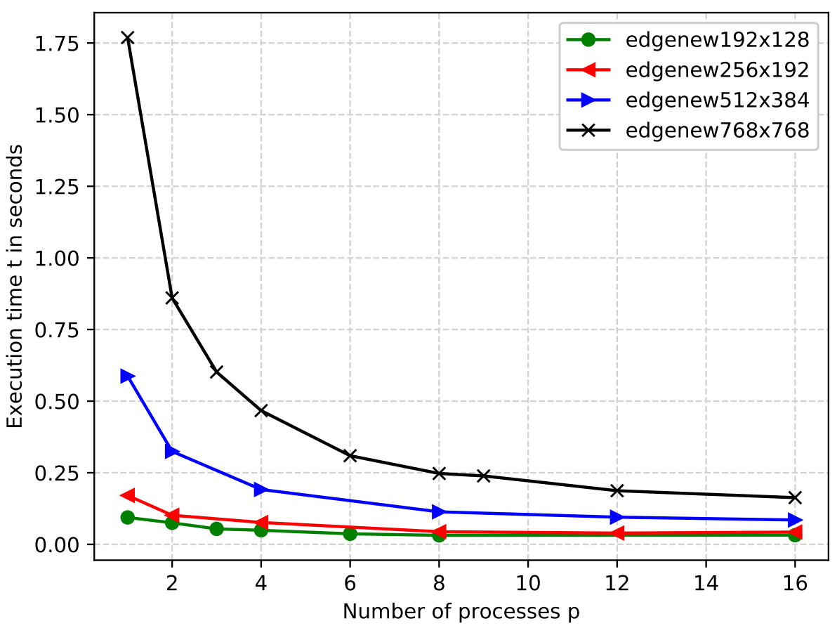
Figure exec1500 shows the execution time for four different input images on one to 16 processes with 1500 iterations. The image with the biggest dimensions takes the longest execution time. The smaller the image dimensions the shorter the execution time. For the same number of processes images of higher edge sizes allocate more pixels per process, resulting in longer execution times with increasing image dimensions.
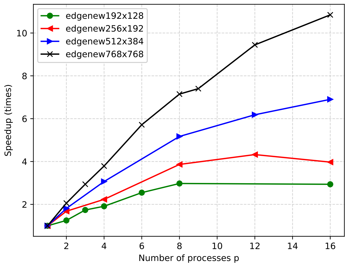
The bigger the image dimensions, the higher our performance gains. Figure speedup1500 shows the speedup for 1500 iterations. The image of size 768x768 reaches a nearly ideal speedup. We ran the experiments thrice and computed averages. Increasing the number of repetitions we could receive more stable results.
Conclusions
Distributing the input edge image, we experimented with various options. It is possible to broadcast the whole input image from root to all processors in the communicator.
Developing a broadcast solution for our edge detection algorithm involves the least code. We read the edge image with pgmread() to masterbuf and MPI_Bcast() sends a copy of the whole M*N image to the other processes. Each process selects a slice of the received image based on its ranks respective coordinates.
We opted for point-to-point communications involving sends on root and receives on non-root processes. As root manages the IO, we let it slice the masterbuf image into dims[0]*dims[1] equally sized parts. dims carries the number of nodes in each dimension set by MPI_Dims_create, i.e. for four processes the routine returns 2*2, for six processes it returns 3*2, for seven processes it returns 7*1 etc. It is a convenient and reasonable option to set up a correct Cartesian topology. An issue arises if the input image cannot directly be split into equally sized slices due to odd numbers of pixels in any dimension. For this edge case, we suggest extending to read the image to the masterbuf array and to extend its size with additional, blank items to reach the next larger size that is dividable by dims[dimension]. Processes receiving parts of the image with “dummy” pixels need to implement an advanced functionality to deal with halo swaps excluding these substitute array items.
Distributing the input image, we can manually slice the image and send it to non-root processes. Figure masterbuf_bufs depicts the example of N=4 processes. masterbuf is divided into four equally sized slices by copying the respective parts to a local buf array with the size MP*NP or M/dims[0] * N/dims[1]. The buf is sent to its respective destinations depending on coordinates of buf as part of the coordination system masterbuf. This option uses data type MPI_Double to send images.
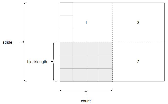
Figure masterbuf_vector shows a second implementation dealing with MPI_Datatypes and MPI_Type_vector. We declare a vector with count MP, blocklength NP and stride N. Taking advantage of this data type we do not have to manually copy slices of masterbuf to buf. Instead, we use MPI_Type_vector(MP, NP, N, MPI_DOUBLE, &vector_distribute) to send slices from root to non-root processes and MPI_Type_vector(MP, NP+2, N, MPI_DOUBLE, &vector_set_edge) to receive on non-root processes to array edge. Instead of copying from buf to edge, the program implements derived datatypes.
We recommend using tags. Writing blocks of non-blocking send statements and blocks of blocking receive statements with a block of MPI_Waits thereafter, the order of receiving is essential. Using tags we increased readability of our implemented logic. Moreover, tags have been very helpful throughout our development for debugging MPI programs.
In section overlapping we presented our performance results for overlapping communications. The difference between execution times for standard and overlapping communication does not significantly increase with an increase in number of processes. In our experiment the results are nearly about the same and differ in less than 0.1 ms. Further investigation could look into scaling on excessive numbers of processes and the impact of network overhead on execution time. Our program and the deployed edge detection algorithm computes reversing values based on four neighbours. It could be interesting to implement an alternative algorithm that e.g. relies on eight neighbours - the four we are using plus the four diagonal pixel neighbours. Increasing the input the for the algorithm we need to add four additional halo swaps. We expect that the advantage of overlapping communication increases with increasing number of halo swaps per iteration or with decreasing network efficiency, respectively higher overheads for one pair of send and receive.